ESG Quick Analysis

Introduction

Candidate

Jose Andres Montes Lopez (preferred name is Andres)

Experience & Skills

• Project Management (Stakeholder exposure & Presentation Skills)
• Data Analysis (Intermediate Python & R, Experience working with Diverse Data sets)
• Demonstrated ESG Interest (Kellog Morgan Stanley Plastic Award Recipient, Social Business Consulting in undergraduate, lead internal Education Pillar in the Social Justice & Impact group)

Context

As part of an upcoming interview, I am preparing a quick analysis of a few funds to highlight basic quantitative and data visualizations using R.

The short analyses below leverage a package called tidyquant that consolidates a variety of analytic, manipulation, and visualization packages. In particular, it provides quick access to a comprehensive set of data sources such as Bloomberg and Yahoo Finance. Another popular feature includes the integration of dplyr facilitating data transformation and manipulation between data visualizations.

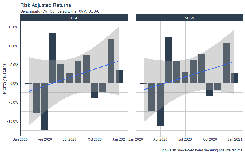
The data used is from Yahoo Finance, and it covers the 2020 calendar year. The funds used in the analysis include three ESG ETFs (SUSA, XVV, ESGU) and a “vanilla” ETF (IVV) that tracks the S&P 500. The latter “vanilla” ETF is the benchmark. In the last chart and table, XVV was switched with ESGU to have a complete year to analyze.

Results

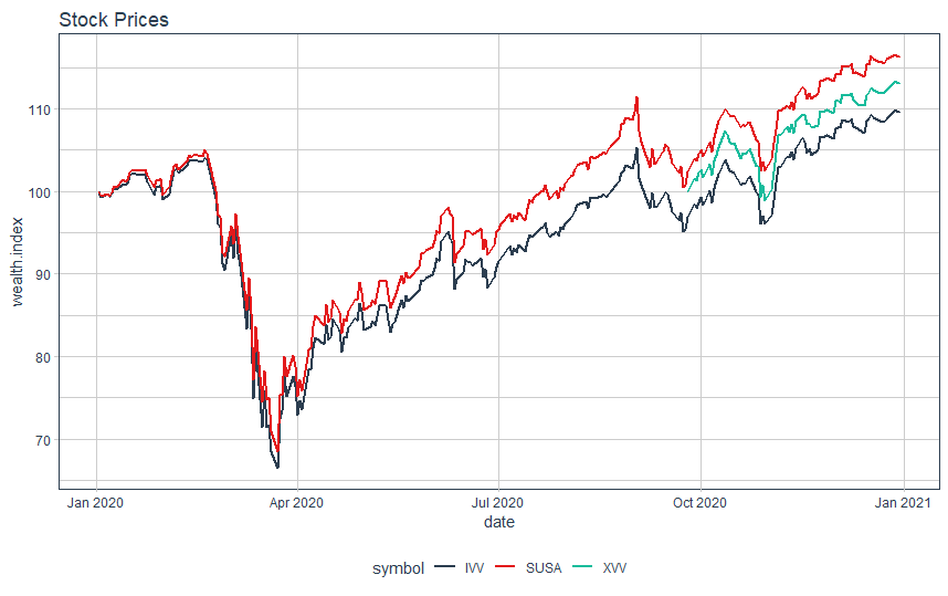
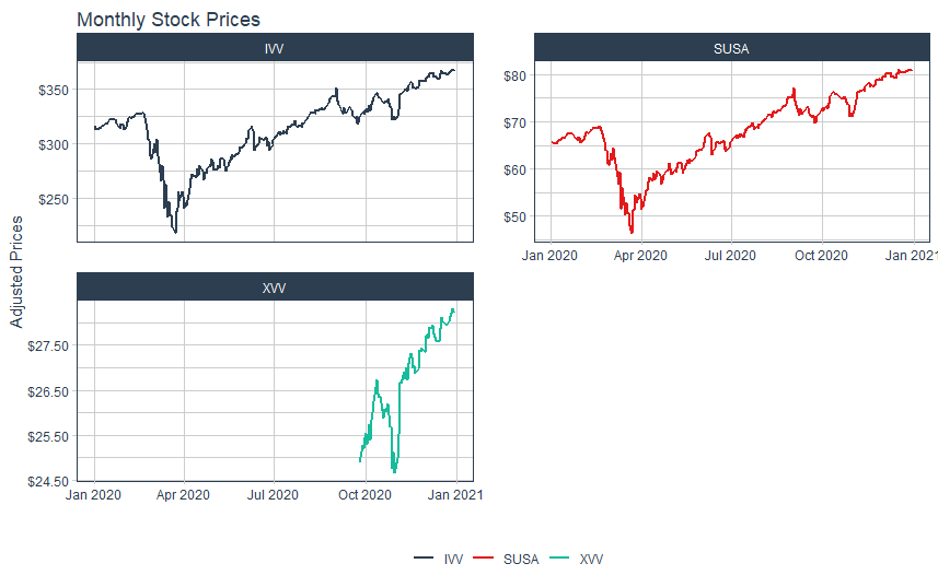
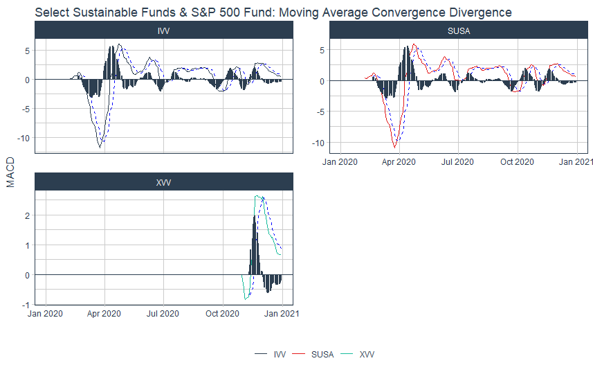
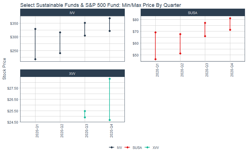
Overall, the charts below show selected ESG ETFs outperformed the benchmark consistently throughout 2020 and signaled opportunities for trading the ETFs. In charts 1,2 and 5 we see ESG ETF outperforming the benchmark. Chart 4 describes the price ranges of the ETFs. Chart 5 visualizes the MACD displaying multiple opportunities to buy/sell the ESG ETFs based on the acceleration of trends between the benchmark and selected ETFs.

Code

Data Import

library(tidyquant)
library(tidyverse)
library(ggplot2)
library(tidyr)
library(dplyr)

stock_prices <- c("SUSA", "IVV","XVV") %>%
    tq_get(get  = "stock.prices",
           from = "2020-01-01",
           to   = "2020-12-31") %>%
    group_by(symbol) 

Data Manipulation Chart 1

stock_prices %>%
    tq_transmute(adjusted, 
                 periodReturn, 
                 period = "daily", 
                 type = "log", 
                 col_rename = "returns") %>%
    mutate(wealth.index = 100 * cumprod(1 + returns)) %>%
    ggplot(aes(x = date, y = wealth.index, color = symbol)) +
    geom_line(size = 1) +
    labs(title = "Stock Prices") +
    theme_tq() + 
    scale_color_tq()

Data Manipulation Chart 2

stock_prices %>%
group_by(symbol) %>%
    tq_transmute(select     = adjusted, 
                 mutate_fun = to.period, 
                 period     = "months")
stock_prices %>%
    ggplot(aes(x = date, y = adjusted, color = symbol)) +
    geom_line(size = 1) +
    labs(title = "Monthly Stock Prices",
         x = "", y = "Adjusted Prices", color = "") +
    facet_wrap(~ symbol, ncol = 2, scales = "free_y") +
    scale_y_continuous(labels = scales::dollar) +
    theme_tq() + 
    scale_color_tq()

Data Manipulation Chart 3

Stock_macd <- stock_prices %>%
    group_by(symbol) %>%
    tq_mutate(select     = close, 
              mutate_fun = MACD, 
              nFast      = 12, 
              nSlow      = 26, 
              nSig       = 9, 
              maType     = SMA) %>%
    mutate(diff = macd - signal) %>%
    select(-(open:volume))
Stock_macd

Stock_macd %>%
    filter(date >= as_date("2016-10-01")) %>%
    ggplot(aes(x = date)) + 
    geom_hline(yintercept = 0, color = palette_light()[[1]]) +
    geom_line(aes(y = macd, col = symbol)) +
    geom_line(aes(y = signal), color = "blue", linetype = 2) +
    geom_bar(aes(y = diff), stat = "identity", color = palette_light()[[1]]) +
    facet_wrap(~ symbol, ncol = 2, scale = "free_y") +
    labs(title = "Select Sustainable Funds & S&P 500 Fund: Moving Average Convergence Divergence",
         y = "MACD", x = "", color = "") +
    theme_tq() +
    scale_color_tq()

Data Manipulation Chart 4

Stock_max_by_qtr <- stock_prices %>%
    group_by(symbol) %>%
    tq_transmute(select     = adjusted, 
                 mutate_fun = apply.quarterly, 
                 FUN        = max, 
                 col_rename = "max.close") %>%
    mutate(year.qtr = paste0(year(date), "-Q", quarter(date))) %>%
    select(-date)
Stock_max_by_qtr

Stock_min_by_qtr <- stock_prices %>%
    group_by(symbol) %>%
    tq_transmute(select     = adjusted, 
                 mutate_fun = apply.quarterly, 
                 FUN        = min, 
                 col_rename = "min.close") %>%
    mutate(year.qtr = paste0(year(date), "-Q", quarter(date))) %>%
    select(-date)

Stock_by_qtr <- left_join(FANG_max_by_qtr, FANG_min_by_qtr,
                         by = c("symbol"   = "symbol",
                                "year.qtr" = "year.qtr"))
Stock_by_qtr

Stock_by_qtr %>%
    ggplot(aes(x = year.qtr, color = symbol)) +
    geom_segment(aes(xend = year.qtr, y = min.close, yend = max.close),
                 size = 1) +
    geom_point(aes(y = max.close), size = 2) +
    geom_point(aes(y = min.close), size = 2) +
    facet_wrap(~ symbol, ncol = 2, scale = "free_y") +
    labs(title = "Select Sustainable Funds & S&P 500 Fund: Min/Max Price By Quarter",
         y = "Stock Price", color = "") +
    theme_tq() +
    scale_color_tq() +
    scale_y_continuous(labels = scales::dollar) +
    theme(axis.text.x = element_text(angle = 90, hjust = 1),
          axis.title.x = element_blank())

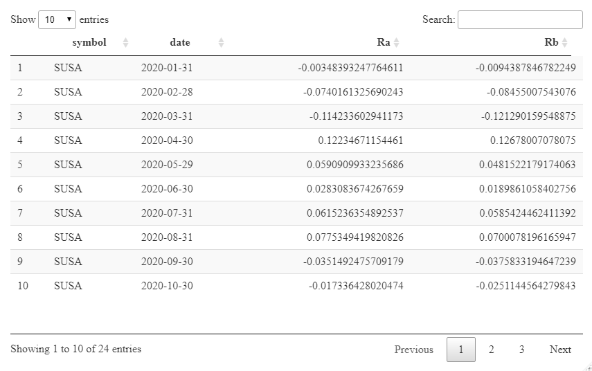
Data Manipulation Table 1

Ra <- c("SUSA", "XVV") %>%
    tq_get(get  = "stock.prices",
           from = "2010-01-01",
           to   = "2015-12-31") %>%
    group_by(symbol) %>%
    tq_transmute(select     = adjusted, 
                 mutate_fun = periodReturn, 
                 period     = "monthly", 
                 col_rename = "Ra")
Ra

Rb <- "IVV" %>%
    tq_get(get  = "stock.prices",
           from = "2010-01-01",
           to   = "2015-12-31") %>%
    tq_transmute(select     = adjusted, 
                 mutate_fun = periodReturn, 
                 period     = "monthly", 
                 col_rename = "Rb")
Rb

RaRb <- left_join(Ra, Rb, by = c("date" = "date"))
RaRb

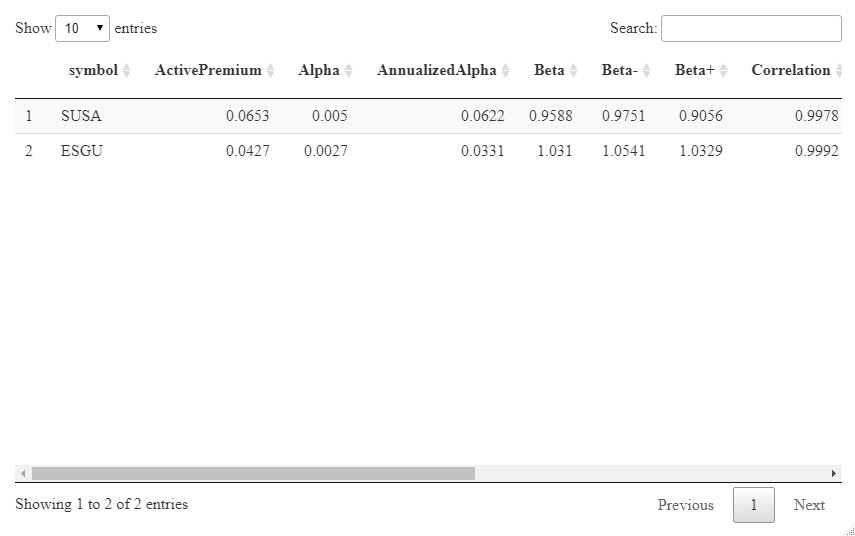
Data Manipulation Table 2

RaRb_capm <- RaRb %>%
    tq_performance(Ra = Ra, 
                   Rb = Rb, 
                   performance_fun = table.CAPM)
RaRb_capm